Configuration Files¶

This page outlines how to construct configuration files to run your own routines with Pipeline.

SkyPy is an astrophysical simulation pipeline tool that allows to define any arbitrary workflow and store data in table format. You may use SkyPy Pipeline to call any function –your own implementation, from any compatible external software or from the SkyPy library. Then SkyPy deals with the data dependencies and provides a library of functions to be used with it.

These guidelines start with an example using one of the SkyPy functions, and it follows the concrete YAML syntax necessary for you to write your own configuration files, beyond using SkyPy functions.

SkyPy example¶

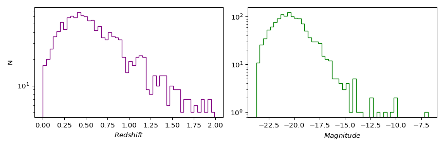
In this section, we exemplify how you can write a configuration file and use some of the SkyPy functions. In this example, we sample redshifts and magnitudes from the SkyPy luminosity function, schechter_lf.

Define variables:

From the documentation, the parameters for the schechter_lf function are: redshift, the characteristic absolute magnitude M_star, the amplitude phi_star, faint-end slope parameter alpha, the magnitude limit magnitude_limit, the fraction of sky sky_area, cosmology and noise. If you are planning to reuse some of these parameters, you can define them at the top-level of your configuration file. In our example, we are using Astropy linear and exponential models for the characteristic absolute magnitude and the amplitude, respectively. Also, noise is an optional parameter and you could use its default value by omitting its definition.

cosmology: !astropy.cosmology.default_cosmology.get []
z_range: !numpy.linspace [0, 2, 21]
M_star: !astropy.modeling.models.Linear1D [-0.9, -20.4]
phi_star: !astropy.modeling.models.Exponential1D [3e-3, -9.7]
magnitude_limit: 23
sky_area: 0.1 deg2

Tables and columns:

You can create a table blue_galaxies and for now add the columns for redshift and magnitude (note here the schechter_lf returns a 2D object)

tables:
  blue_galaxies:
    redshift, magnitude: !skypy.galaxies.schechter_lf
      redshift: $z_range
      M_star: $M_star
      phi_star: $phi_star
      alpha: -1.3
      m_lim: $magnitude_limit
      sky_area: $sky_area

Important: if cosmology is detected as a parameter but is not set, it automatically uses the cosmology variable defined at the top-level of the file.

This is how the entire configuration file looks like!

cosmology: !astropy.cosmology.default_cosmology.get []
z_range: !numpy.linspace [0, 2, 21]
M_star: !astropy.modeling.models.Linear1D [-0.9, -20.4]
phi_star: !astropy.modeling.models.Exponential1D [3e-3, -9.7]
magnitude_limit: 23
sky_area: 0.1 deg2
tables:
  blue_galaxies:
    redshift, magnitude: !skypy.galaxies.schechter_lf
      redshift: $z_range
      M_star: $M_star
      phi_star: $phi_star
      alpha: -1.3
      m_lim: $magnitude_limit
      sky_area: $sky_area

You may now save it as luminosity.yml and run it using the SkyPy Pipeline:

import matplotlib.pyplot as plt
from skypy.pipeline import Pipeline

# Execute SkyPy luminosity pipeline
pipeline = Pipeline.read("luminosity.yml")
pipeline.execute()

# Blue population
skypy_galaxies = pipeline['blue_galaxies']

# Plot histograms
fig, axs = plt.subplots(1, 2, figsize=(9, 3))

axs[0].hist(skypy_galaxies['redshift'], bins=50, histtype='step', color='purple')
axs[0].set_xlabel(r'$Redshift$')
axs[0].set_ylabel(r'$\mathrm{N}$')
axs[0].set_yscale('log')

axs[1].hist(skypy_galaxies['magnitude'], bins=50, histtype='step', color='green')
axs[1].set_xlabel(r'$Magnitude$')
axs[1].set_yscale('log')

plt.tight_layout()
plt.show()

You can also run the pipeline directly from the command line and write the outputs to a fits file:

$ skypy luminosity.yml luminosity.fits

Don’t forget to check out for more complete examples!

YAML syntax¶

YAML is a file format designed to be readable by both computers and humans. Fundamentally, a file written in YAML consists of a set of key-value pairs. Each pair is written as key: value, where whitespace after the : is optional. The hash character # denotes the start of a comment and all further text on that line is ignored by the parser.

This guide introduces the main syntax of YAML relevant when writing a configuration file to use with SkyPy. Essentially, it begins with definitions of individual variables at the top level, followed by the tables, and, within the table entries, the features of objects to simulate are included. Main keywords: parameters, cosmology, tables.

Variables¶

Variable definition: a variable is defined as a key-value pair at the top of the file. YAML is able to interpret any numeric data with the appropriate type: integer, float, boolean. Similarly for lists and dictionaries. In addition, SkyPy has added extra functionality to interpret and store Astropy Quantities. Everything else is stored as a string (with or without explicitly using quotes)
```
# YAML interprets
counter: 100 # An integer
miles: 1000.0 # A floating point
name: "Joy" # A string
planet: Earth # Another string
mylist: [ 'abc', 789, 2.0e3 ] # A list
mydict: { 'fruit': 'orange', 'year': 2020 } # A dictionary

# SkyPy extra functionality
angle: 10 deg
distance: 300 kpc
```
Import objects: the SkyPy configuration syntax allows objects to be imported directly from external (sub)modules using the ! tag and providing neither a list of arguments or a dictionary of keywords. For example, this enables the import and usage of any Astropy cosmology:
```
cosmology: !astropy.cosmology.Planck13 # import the Planck13 object and bind it to the variable named "cosmology"
```

Parameters¶

Parameters definition: parameters are variables that can be modified at execution.

For example,
```
parameters:
  hubble_constant: 70
  omega_matter: 0.3
```

Functions¶

Function call: functions are defined as tuples where the first entry is the fully qualified function name tagged with and exclamation mark ! and the second entry is either a list of positional arguments or a dictionary of keyword arguments.

For example, if you need to call the log10() and linspace() NumPy functions, then you define the following key-value pairs:
```
log_of_2: !numpy.log10 [2]
myarray: !numpy.linspace [0, 2.5, 10]
```
You can also define parameters of functions with a dictionary of keyword arguments. Imagine you want to compute the comoving distance for a range of redshifts and an Astropy Planck 2015 cosmology. To run it with the SkyPy pipeline, call the function and define the parameters as an indented dictionary.
```
comoving_distance: !astropy.cosmology.Planck15.comoving_distance
  z: !numpy.linspace [ 0, 1.3, 10 ]
```
Similarly, you can specify the functions arguments as a dictionary:
```
comoving_distance: !astropy.cosmology.Planck15.comoving_distance
  z: !numpy.linspace {start: 0, stop: 1.3, num: 10}
```
N.B. To call a function with no arguments, you should pass an empty list of args or an empty dictionary of kwargs. For example:
```
cosmo: !astropy.cosmology.default_cosmology.get []
```
Variable reference: variables can be referenced by their full name tagged with a dollar sign $. In the previous example you could also define the variables at the top-level of the file and then reference them:
```
redshift: !numpy.linspace [ 0, 1.3, 10 ]
comoving_distance: !astropy.cosmology.Planck15.comoving_distance
  z: $redshift
```
The cosmology to be used by functions within the pipeline only needs to be set up at the top. If a function needs cosmology as an input, you need not define it again, it is automatically detected.

For example, calculate the angular size of a galaxy with a given physical size, at a fixed redshift and for a given cosmology:
```
cosmology: !astropy.cosmology.FlatLambdaCDM
  H0: 70
  Om0: 0.3
size: !skypy.galaxies.morphology.angular_size
  physical_size: 10 kpc
  redshift: 0.2
```
Job completion: .depends can be used to force any function call to wait for completion of any other job.

A simple example where, for some reason, the comoving distance needs to be called after completion of the angular size function:
```
cosmology: !astropy.cosmology.Planck15
size: !skypy.galaxies.morphology.angular_size
  physical_size: 10 kpc
  redshift: 0.2
comoving_distance: !astropy.cosmology.Planck15.comoving_distance
  z: !numpy.linspace [ 0, 1.3, 10 ]
  .depends: size
```
By doing so, you force the function call redshift to be completed before is used to compute the comoving distance.

Tables¶

Table creation: a dictionary of table names, each resolving to a dictionary of column names for that table.

Let us create a table called telescope with a column to store the width of spectral lines that follow a normal distribution
```
tables:
  telescope:
    spectral_lines: !scipy.stats.norm.rvs
      loc: 550
      scale: 1.6
      size: 100
```

Column addition: you can add as many columns to a table as you need.: Imagine you want to add a column for the telescope collecting surface

tables:
  telescope:
    spectral_lines: !scipy.stats.norm.rvs
      loc: 550
      scale: 1.6
      size: 100
    collecting_surface: !numpy.random.uniform
      low: 6.9
      high: 7.1
      size: 100

Column reference: columns in the pipeline can be referenced by their full name tagged with a dollar sign $. Example: the galaxy mass that follows a lognormal distribution. You can create a table galaxies with a column mass where you sample 10000 object and a second column, radius which also follows a lognormal distribution but the mean depends on how massive the galaxies are:
```
tables:
  galaxies:
    mass: !numpy.random.lognormal
      mean: 5.
      size: 10000
    radius: !numpy.random.lognormal
      mean: $galaxies.mass
```
Multi-column assignment: multi-column assignment is performed with any 2d-array, where one of the dimensions is interpreted as the rows of the table and the second dimension, as separate columns. Or you can do it from a function that returns a tuple.

We use multi-column assignment in the following example where we sample a two-dimensional array of values from a lognormal distribution and then store them as three columns in a table:
```
tables:
  halos:
    mass, radius, concentration: !numpy.random.lognormal
      size: [10000, 3]
```
Table initialisation: by default tables are initialised using astropy.table.Table() however this can be overridden using the .init keyword to initialise the table with any function call.

For example, you can stack galaxy properties such as radii and mass:
```
radii: !numpy.logspace [ 1, 2, 100 ]
mass: !numpy.logspace [ 9, 12, 100 ]
tables:
  galaxies:
    .init: !astropy.table.vstack [[ $radii, $mass ]]
```
Table reference: when a function call depends on tables, you need to ensure the referenced table has the necessary content and is not empty. You can do that with .complete.

Example: you want to perform a very simple abundance matching, i.e. painting galaxies within your halos. You can create two tables halos and galaxies storing the halo mass and galaxy luminosities. Then you can stack these two tables and store it in a third table called matching.
```
tables:
  halos:
    halo_mass: !numpy.random.uniform
      low: 1.0e8
      high: 1.0e14
      size: 20
  galaxies:
    luminosity: !numpy.random.uniform
      low: 0.05
      high: 10.0
      size: 20
  matching:
    .init: !astropy.table.hstack
      tables: [ $halos, $galaxies ]
      .depends: [ halos.complete, galaxies.complete ]
```

Navigation